Examples
Running Python gaussdecomp
Here’s an example of running Python gaussdecomp on a GBT datacube.
from gaussdriver import driver
gstruc = driver.driver('mycube.fits',368,8)
RUNNING GAUSSIAN ANALYSIS WITH THE FOLLOWING PARAMETERS
-----------------------------------------------------------
STARTING POSITION = (368,8)
X RANGE = [0,499]
Y RANGE = [0,249]
X DIRECTION = 1
Y DIRECTION = 1
OUTFILE = gaussdecomp_20220329165135.fits
-----------------------------------------------------------
USING (BACKRET) MODE
-----------------------------------------------------------

Fitting Gaussians to the HI spectrum at (368,8)
FORWARD
Zero-velocity region INCLUDED.  Fitting it separately
Attempting to remove small Gaussians
Attempting to remove small Gaussians
----------------------------------------------------------
#       Height         Center         Width       Area
----------------------------------------------------------
1   24.11 (0.47)  -2.30 (0.04)   6.23 (0.07) 376.64
2    3.95 (0.12) -36.17 (0.59)  32.14 (0.50) 317.88
3   12.63 (0.14) -44.70 (0.09)   5.62 (0.13) 177.83
4    7.99 (0.77)  -1.91 (0.37)   2.24 (0.27)  44.89
5    5.05 (0.15) -30.43 (0.11)   3.13 (0.12)  39.63
6    2.92 (0.15) -58.41 (0.38)   4.38 (0.31)  32.01
7    8.62 (1.35)   1.51 (0.14)   1.46 (0.10)  31.49
8    0.81 (0.02) 590.60 (15.05) 256.46 (9.09) 520.46
----------------------------------------------------------
RMS = 0.085
Noise = 0.250
dt = 1.5 sec

Last/Current Position = (368,8)
Neighbors (position)  visited  better  redo
P1 (  369,    8)        0       -1    False
P2 (  368,    9)        0       -1    False
P3 (  367,    8)        0       -1    False
P4 (  368,    7)        0       -1    False

Fitting Gaussians to the HI spectrum at (369,8)
FORWARD
Zero-velocity region INCLUDED.  Fitting it separately
Attempting to remove small Gaussians
Attempting to remove small Gaussians
----------------------------------------------------------
#       Height         Center         Width       Area
----------------------------------------------------------
1   29.60 (0.23)  -2.44 (0.05)   5.77 (0.04) 428.43
2    4.54 (0.15) -34.18 (0.71)  31.46 (0.59) 357.99
3   10.24 (0.49) -43.71 (0.30)   4.66 (0.34) 119.56
4    4.11 (0.39) -55.35 (1.20)   5.76 (0.75)  59.36
5    3.89 (0.26) -31.85 (0.38)   3.66 (0.35)  35.66
6    8.63 (0.30)   0.97 (0.05)   1.63 (0.07)  35.21
7    0.83 (0.02) 590.60 (18.42) 251.09 (11.13) 519.35
----------------------------------------------------------
RMS = 0.107
Noise = 0.217
dt = 1.7 sec

Count = 2
Last/Current Position = (369,8)
Neighbors (position)  visited  better  redo
P1 (  370,    8)        0       -1    False
P2 (  369,    9)        0       -1    False
P3 (  368,    8)        1        0     True
P4 (  369,    7)        0       -1    False

Fitting Gaussians to the HI spectrum at (368,8)
REDO FORWARD
Zero-velocity region INCLUDED.  Fitting it separately
Using First Guess Parameters
Attempting to remove small Gaussians
----------------------------------------------------------
#       Height         Center         Width       Area
----------------------------------------------------------
1    0.80 (0.04) 590.60 (40.21) 262.92 (25.62) 528.29
2    4.82 (0.11) -35.69 (0.49)  31.23 (0.50) 377.43
3   33.06 (0.20)  -0.93 (0.08)   4.53 (0.05) 375.46
4   11.02 (0.13) -45.20 (0.07)   6.81 (0.10) 187.98
5    6.24 (0.42)  -9.68 (0.28)   3.36 (0.18)  52.58
6    3.91 (0.18) -30.00 (0.11)   2.14 (0.12)  20.96
----------------------------------------------------------
RMS = 0.202
Noise = 0.250
dt = 1.8 sec

Count = 3
Last/Current Position = (368,8)
Neighbors (position)  visited  better  redo
P1 (  369,    8)        1        0     True
P2 (  368,    9)        0       -1    False
P3 (  367,    8)        0       -1    False
P4 (  368,    7)        0       -1    False

Fitting Gaussians to the HI spectrum at (369,8)
REDO FORWARD
Zero-velocity region INCLUDED.  Fitting it separately
Attempting to remove small Gaussians
Attempting to remove small Gaussians
----------------------------------------------------------
#       Height         Center         Width       Area
----------------------------------------------------------
1   29.60 (0.23)  -2.44 (0.05)   5.77 (0.04) 428.43
2    4.54 (0.15) -34.18 (0.71)  31.46 (0.59) 357.99
3   10.24 (0.49) -43.71 (0.30)   4.66 (0.34) 119.56
4    4.11 (0.39) -55.35 (1.20)   5.76 (0.75)  59.36
5    3.89 (0.26) -31.85 (0.38)   3.66 (0.35)  35.66
6    8.63 (0.30)   0.97 (0.05)   1.63 (0.07)  35.21
7    0.83 (0.02) 590.60 (18.42) 251.09 (11.13) 519.35
----------------------------------------------------------
RMS = 0.107
Noise = 0.217
dt = 1.6 sec
Running IDL gaussdecomp
The main program is gdriver.pro. I normally create a small IDL batch script to run segments of a cube. An example one is provided using a small GASS (McClure-Griffiths et al. 2009) cube downloaded from https://www.astro.uni-bonn.de/hisurvey/gass/ using these parameters:
l = 295.0 deg
b = -41.0 deg
width in l = 1 deg
width in b = 1 deg
The example script is gass.in and looks like this:
spawn,'echo $HOST',host
print,'RUNNING THIS PROGRAM ON ',host
@compile_all
; The cube is [13,13,1201]
gdriver,lonr=[0,12],latr=[0,12],cubefile='../gass_295_-41.fits.gz',file='gass.fits',/noplot,$
    btrack=btrack,gstruc=gstruc,/backret,savestep=100
Run it like this:
idl
IDL>@gass.in
The output should look something like this:
IDL>@gass.in
RUNNING THIS PROGRAM ON  NideverMacBookPro-2.local
RUNNING GAUSSIAN ANALYSIS WITH THE FOLLOWING PARAMETERS
-----------------------------------------------------------
% Compiled module: STRINGIZE.
% Compiled module: STRMULT.
STARTING POSITION = (0.0,0.0)
LONGITUDE RANGE = [0.0,12.0]
LATITUDE RANGE = [0.0,12.0]
LON DIRECTION = 1
LAT DIRECTION = 1
FILE = gass.fits
-----------------------------------------------------------
USING (BACKRET) MODE
-----------------------------------------------------------

Fitting Gaussians to the HI spectrum at (0.0,0.0)
FORWARD
% Compiled module: UNDEFINE.
LOADING DATACUBE from ../data/gass_295_-41.fits.gz
X = GLON-CAR  [X] = 13
Y = GLAT-CAR  [Y] = 13
Z = VELO-LSRK  [Z] = 1201
Converting m/s to km/s

----------------------------------------------------------
#       Height         Center         Width       Area
----------------------------------------------------------
1     2.60 ( 4.5)   -2.48 ( 4.4)   11.52 ( 5.5)   75.04
2     5.12 (  18)   -1.84 (  26)    5.47 (  11)   70.11
3     2.84 (  51)    9.51 (  63)    3.09 (  19)   21.96
4     4.98 ( 8.8)   -2.82 (0.91)    1.52 (1.00)   18.98
5     2.92 (  73)    7.42 ( 6.1)    1.96 (  11)   14.35
6     2.08 (  25)    1.56 ( 5.8)    1.75 ( 7.6)    9.15
7     5.98 (0.68)  172.13 ( 2.6)   22.14 ( 2.2)  332.19
8     6.64 ( 4.6)  151.59 ( 3.1)    5.44 ( 2.8)   90.57
9     5.05 ( 1.7)  181.76 (0.88)    5.04 ( 1.2)   63.82
10     4.77 ( 4.6)  151.87 (0.66)    2.49 ( 1.2)   29.80
11     3.26 ( 1.8)  180.39 (0.59)    1.98 (0.87)   16.17
12     0.98 (0.39)  217.66 ( 2.5)    5.70 ( 2.8)   13.94
13     1.93 ( 2.1)  139.48 (  10)    5.55 ( 5.5)   26.84
----------------------------------------------------------
RMS = 0.0523
Noise = 0.0490

Count = 1
Last/Current Position = (0.0,0.0)
Neighbors (position)  visited  better  redo
P1  (  1.0,  0.0)        -1      -1       0
P2  (  0.0,  1.0)        -1      -1       0
P3  (-----,-----)        -1      -1       0
P4  (-----,-----)        -1      -1       0

Fitting Gaussians to the HI spectrum at (1.0,0.0)
FORWARD
----------------------------------------------------------
#       Height         Center         Width       Area
----------------------------------------------------------
1     2.86 ( 6.5)   -2.02 ( 4.0)   11.26 ( 6.3)   80.62
2     4.85 (  22)   -2.07 (  32)    5.50 (  15)   66.80
3     5.18 (  10)   -2.97 (0.67)    1.51 (0.92)   19.58
4     2.55 (  37)    9.70 (  54)    2.96 (  18)   18.98
5     2.85 (  66)    7.33 ( 5.7)    1.93 (  10)   13.79
6     2.21 (  33)    1.63 ( 4.6)    1.83 ( 8.8)   10.13
7     6.81 ( 2.7)  174.45 (  18)   16.71 (  19)  285.34
8    13.49 (  14)  151.51 ( 3.2)    3.12 ( 1.6)  105.34
9     4.08 (  14)  144.58 (  34)    8.42 (  17)   86.08
10     5.31 ( 3.6)  181.15 ( 1.3)    4.50 ( 2.3)   59.94
11     3.28 (  17)  157.44 (  15)    3.42 ( 8.4)   28.16
12     1.22 ( 1.4)  216.15 (  13)    9.12 (  10)   27.79
13     3.51 ( 2.8)  179.84 (0.71)    1.98 (1.00)   17.41
14     0.28 (0.36)  116.95 (  51)   13.09 (  36)    9.31
15     0.96 ( 6.2)  144.33 ( 5.5)    2.17 ( 6.4)    5.25
16     0.49 ( 1.2)  217.88 ( 4.1)    2.93 ( 6.6)    3.62
----------------------------------------------------------
RMS = 0.0514
Noise = 0.0484

Count = 2
Last/Current Position = (1.0,0.0)
Neighbors (position)  visited  better  redo
P1  (  2.0,  0.0)        -1      -1       0
P2  (  1.0,  1.0)        -1      -1       0
P3  (  0.0,  0.0)        -1      -1       0
P4  (-----,-----)        -1      -1       0

Fitting Gaussians to the HI spectrum at (2.0,0.0)
FORWARD
----------------------------------------------------------
#       Height         Center         Width       Area
----------------------------------------------------------
1     6.01 ( 6.9)   -0.69 ( 3.4)    9.19 ( 4.3)  138.55
2     3.73 ( 6.8)   -1.50 ( 2.0)    3.80 ( 3.0)   35.56
3     3.13 ( 2.9)    8.28 (0.90)    2.49 ( 1.3)   19.54
4     3.54 ( 1.7)   -3.24 (0.39)    1.21 (0.56)   10.76
5     0.19 (0.56)  -26.02 (  37)    6.72 (  26)    3.20
6     7.28 (  12)  151.24 ( 5.8)   10.06 ( 6.5)  183.58
7     7.18 ( 8.1)  178.36 ( 3.5)    7.51 ( 5.3)  135.15
8     2.79 ( 8.1)  182.65 ( 100)   22.82 (  32)  159.41
9     9.79 (  12)  152.97 ( 2.7)    3.89 ( 1.4)   95.51
10     6.20 ( 4.1)  179.46 (0.47)    2.73 ( 1.0)   42.40
11     5.85 (  13)  151.20 ( 1.3)    2.54 ( 1.7)   37.23
12     0.34 (0.77)  112.58 (  50)   13.71 (  28)   11.60
13     1.08 (0.70)  218.13 ( 2.4)    4.74 ( 3.4)   12.84
14     1.15 ( 1.5)  185.70 ( 2.0)    1.74 ( 2.1)    5.03
----------------------------------------------------------
RMS = 0.0572
Noise = 0.0489
On my laptop the example datacube ran for 8 minutes. The resulting file is called gass.fits and availabe in the data/ directory, gzip-compressed.
Output catalog
The final example catalog contains 1923 Gaussians. This is what the columns in the output catalog look like.
LON             FLOAT           2.00000
LAT             FLOAT           1.00000
RMS             FLOAT         0.0505933
NOISE           FLOAT         0.0490385
PAR             FLOAT     Array[3]
SIGPAR          FLOAT     Array[3]
GLON            FLOAT           295.424
GLAT            FLOAT          -41.4000
The columns are:
Column |
Description |
|---|---|
LON |
X position in the grid starting with 0 |
LAT |
Y position in the grid starting with 0 |
RMS |
RMS of the residuals |
NOISE |
Noise level of the spectrum |
PAR |
Gaussian parameters [height, center, sigma] |
SIGPAR |
Uncertainties in PAR |
GLON |
Galactic longitude (or RA) for this position |
GLAT |
Galactic latitude (or DEC) for this position |
Plotting the Results
The repository includes a plotting routine called ghess.pro which is useful for general figures using the catalog of Gaussians.
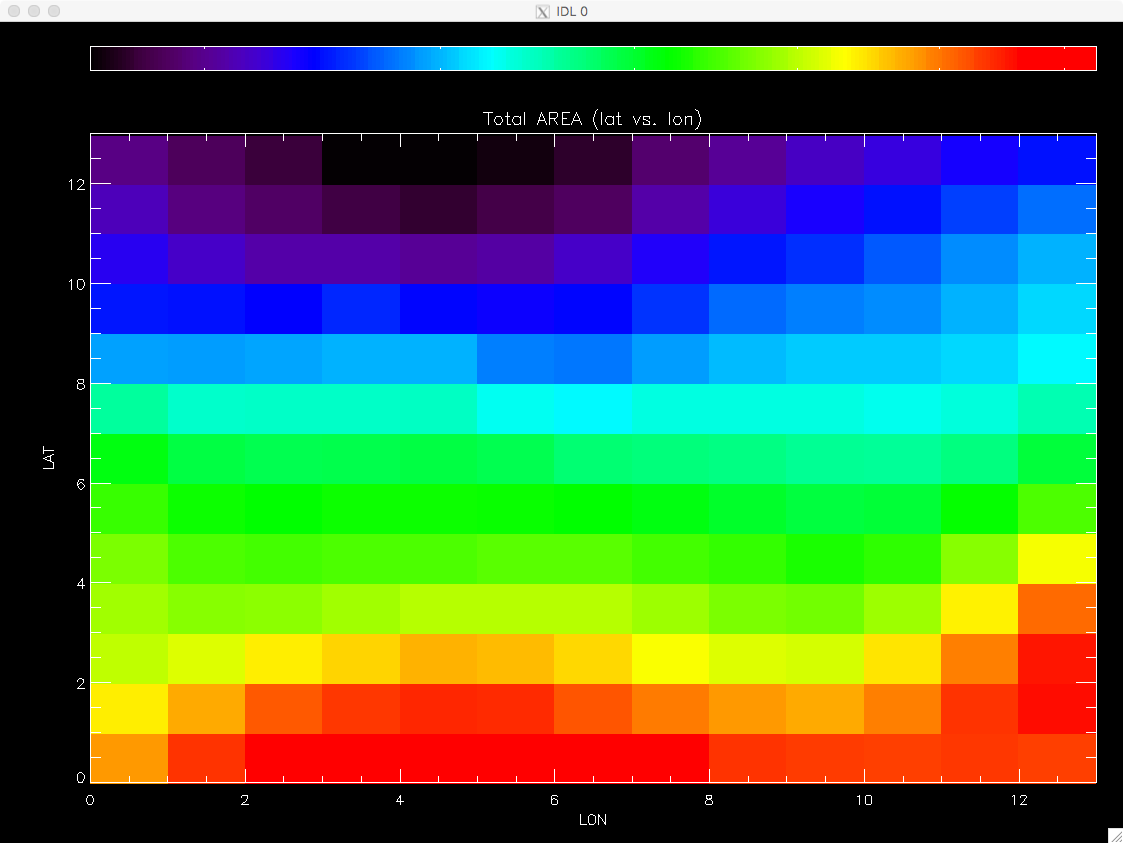
Here’s a simple figure just showing the total area of all the Gaussians in a given, essentially a column density map.
IDL>str = mrdfits('../data/gass.fits.gz',1)
IDL>ghess,str,'lon','lat',dx=1,dy=1,/total,/log
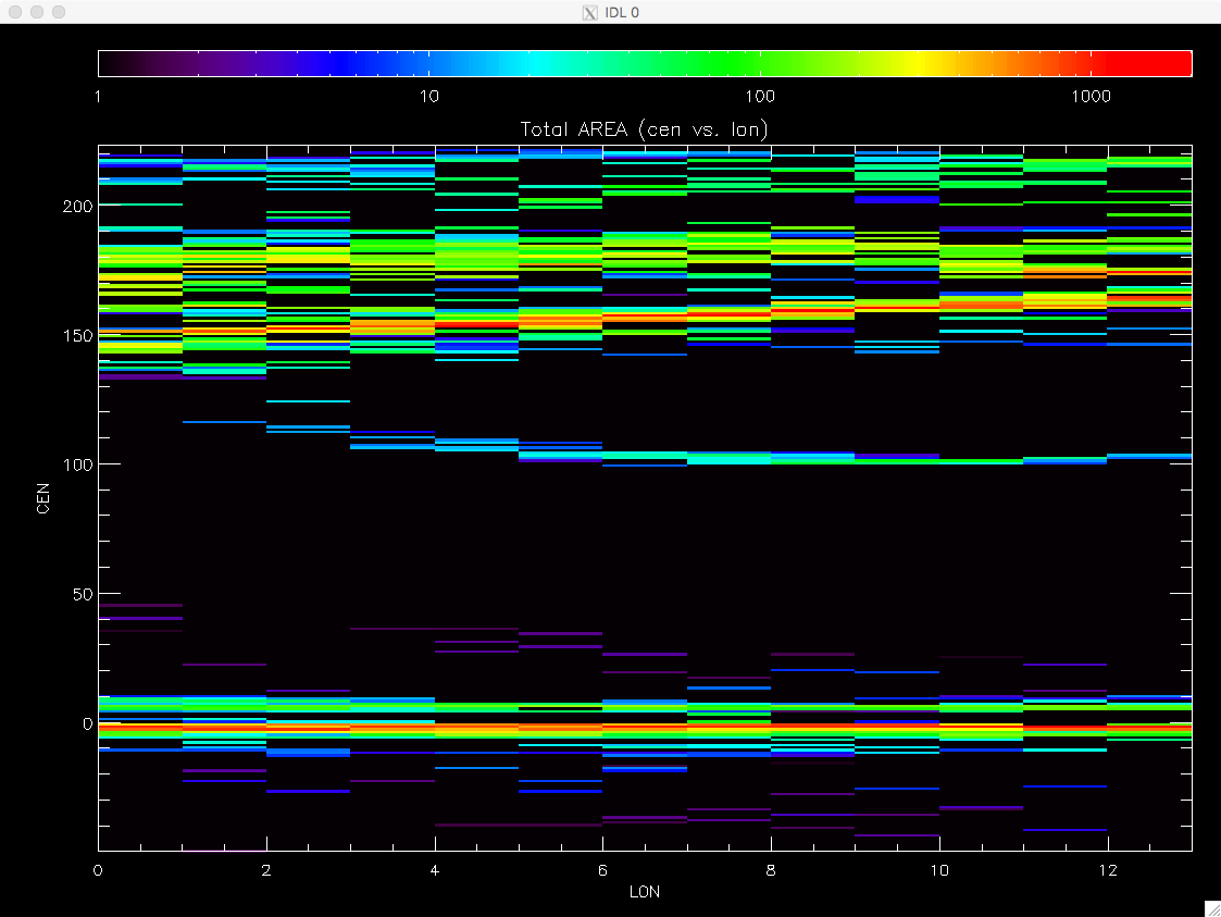
Now let’s plot the velocity of the Gaussian versus one of the coordinates and color-coded by the total area.
IDL>ghess,str,'lon','cen',dx=1,dy=1,/total,/log
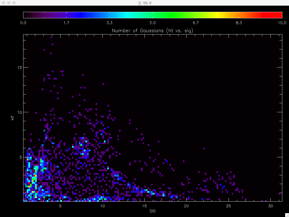
And, finally, we can also plot the distribution of the other Gaussian parameters. Height versus sigma width.
IDL>ghess,str,'sig','ht',dx=0.2,dy=0.2